Support Vector Machine (SVM) - ML Program

 

SVM Classifier for IRIS Data Set

Steps:

1. Import the library files
2. Read the dataset (Iris Dataset) and analyze the data
3. Preprocessing the data
4. Divide the data into Training and Testing
5. Build the model - SVM Classifier with different types of kernels
6. Model Evaluation

1.Import the library files

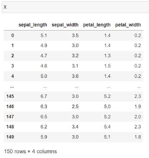
2. Read the dataset (Iris Dataset) and analyze the data

3. Preprocessing the data

4. Divide the data into Training and Testing

5. Build the model - SVM Classifier with different types of kernels

Support vector machines (SVMs) are a set of supervised learning methods used for classification, regression and outliers detection.

The advantages of support vector machines are:

• Effective in high dimensional spaces.

• Still effective in cases where number of dimensions is greater than the number of samples.

• Uses a subset of training points in the decision function (called support vectors), so it is also memory efficient.

• Versatile: different Kernel functions can be specified for the decision function. Common kernels are provided, but it is also possible to specify custom kernels.

The disadvantages of support vector machines include:

• If the number of features is much greater than the number of samples, avoid over-fitting in choosing Kernel functions and regularization term is crucial.

• SVMs do not directly provide probability estimates, these are calculated using an expensive five-fold cross-validation.

class sklearn.svm.SVC(*, C=1.0, kernel='rbf', degree=3, gamma='scale', coef0=0.0, shrinking=True, probability=False, tol=0.001, cache_size=200, class_weight=None, verbose=False, max_iter=-1, decision_function_shape='ovr', break_ties=False, random_state=None)

Parameters:

Cfloat, default=1.0
Regularization parameter. The strength of the regularization is inversely proportional to C. Must be strictly positive. The penalty is a squared l2 penalty.
kernel{‘linear’, ‘poly’, ‘rbf’, ‘sigmoid’, ‘precomputed’} or callable, default=’rbf’
Specifies the kernel type to be used in the algorithm. If none is given, ‘rbf’ will be used. If a callable is given it is used to pre-compute the kernel matrix from data matrices; that matrix should be an array of shape (n_samples, n_samples).
degreeint, default=3
Degree of the polynomial kernel function (‘poly’). Ignored by all other kernels.
gamma{‘scale’, ‘auto’} or float, default=’scale’
Kernel coefficient for ‘rbf’, ‘poly’ and ‘sigmoid’.

if gamma='scale' (default) is passed then it uses 1 / (n_features * X.var()) as value of gamma,
if ‘auto’, uses 1 / n_features.

Changed in version 0.22: The default value of gamma changed from ‘auto’ to ‘scale’.

coef0float, default=0.0

Independent term in kernel function. It is only significant in ‘poly’ and ‘sigmoid’.

shrinkingbool, default=True

Whether to use the shrinking heuristic. 

probabilitybool, default=False

Whether to enable probability estimates. This must be enabled prior to calling fit, will slow down that method as it internally uses 5-fold cross-validation, and predict_proba may be inconsistent with predict.

tolfloat, default=1e-3

Tolerance for stopping criterion.

cache_sizefloat, default=200

Specify the size of the kernel cache (in MB).

class_weightdict or ‘balanced’, default=None

Set the parameter C of class i to class_weight[i]*C for SVC. If not given, all classes are supposed to have weight one. The “balanced” mode uses the values of y to automatically adjust weights inversely proportional to class frequencies in the input data as n_samples / (n_classes * np.bincount(y)).

verbosebool, default=False

Enable verbose output. Note that this setting takes advantage of a per-process runtime setting in libsvm that, if enabled, may not work properly in a multithreaded context.

max_iterint, default=-1

Hard limit on iterations within solver, or -1 for no limit.

decision_function_shape{‘ovo’, ‘ovr’}, default=’ovr’

Whether to return a one-vs-rest (‘ovr’) decision function of shape (n_samples, n_classes) as all other classifiers, or the original one-vs-one (‘ovo’) decision function of libsvm which has shape (n_samples, n_classes * (n_classes - 1) / 2). However, note that internally, one-vs-one (‘ovo’) is always used as a multi-class strategy to train models; an ovr matrix is only constructed from the ovo matrix. The parameter is ignored for binary classification.

Changed in version 0.19: decision_function_shape is ‘ovr’ by default.

New in version 0.17: decision_function_shape=’ovr’ is recommended.

Changed in version 0.17: Deprecated decision_function_shape=’ovo’ and None.

break_tiesbool, default=False

If true, decision_function_shape='ovr', and number of classes > 2, predict will break ties according to the confidence values of decision_function; otherwise the first class among the tied classes is returned. Please note that breaking ties comes at a relatively high computational cost compared to a simple predict.

random_stateint, RandomState instance or None, default=None

Controls the pseudo random number generation for shuffling the data for probability estimates. Ignored when probability is False. Pass an int for reproducible output across multiple function calls. 

a. Linear Kernel 

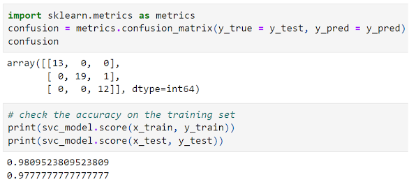
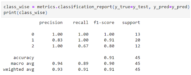
6. SVM- Linear Kernel Model Evaluation

5 & 6 Build the model - SVM RBF Kernel  & Model Evaluation

5 & 6 Build the model - SVM POLY Kernel  & Model Evaluation

KNN Machine Learning Program

KNN Classifier for IRIS Data Set

Steps:

1. Import the library files
2. Read the dataset (Iris Dataset) and analyze the data
3. Preprocessing the data
4. Divide the data into Training and Testing
5. Build the model - KNN Classifier
6. Model Evaluation

1. Import the library files

2. Read the dataset (Iris Dataset) and analyze the data

3. Preprocessing the data

 

4. Divide the data into Training and Testing

5. Build the model - KNN Classifier

KNN Classifier

class sklearn.neighbors.KNeighborsClassifier(n_neighbors=5, *, weights='uniform', algorithm='auto', leaf_size=30, p=2, metric='minkowski', metric_params=None, n_jobs=None)

Parameters:

n_neighborsint, default=5

Number of neighbors to use by default for kneighbors queries.

weights{‘uniform’, ‘distance’} or callable, default=’uniform’

Weight function used in prediction. Possible values:

• ‘uniform’ : uniform weights. All points in each neighborhood are weighted equally.

• ‘distance’ : weight points by the inverse of their distance. in this case, closer neighbors of a query point will have a greater influence than neighbors which are further away.

• [callable] : a user-defined function which accepts an array of distances, and returns an array of the same shape containing the weights.

algorithm{‘auto’, ‘ball_tree’, ‘kd_tree’, ‘brute’}, default=’auto’

Algorithm used to compute the nearest neighbors:

• ‘ball_tree’ will use BallTree

• ‘kd_tree’ will use KDTree

• ‘brute’ will use a brute-force search.

• ‘auto’ will attempt to decide the most appropriate algorithm based on the values passed to fit method.

Note: fitting on sparse input will override the setting of this parameter, using brute force.

leaf_sizeint, default=30

Leaf size passed to BallTree or KDTree. This can affect the speed of the construction and query, as well as the memory required to store the tree. The optimal value depends on the nature of the problem.

pint, default=2

Power parameter for the Minkowski metric. When p = 1, this is equivalent to using manhattan_distance (l1), and euclidean_distance (l2) for p = 2. For arbitrary p, minkowski_distance (l_p) is used.

metricstr or callable, default=’minkowski’

Metric to use for distance computation. Default is “minkowski”, which results in the standard Euclidean distance when p = 2. See the documentation of scipy.spatial.distance and the metrics listed in distance_metrics for valid metric values.

If metric is “precomputed”, X is assumed to be a distance matrix and must be square during fit. X may be a sparse graph, in which case only “nonzero” elements may be considered neighbors.

If metric is a callable function, it takes two arrays representing 1D vectors as inputs and must return one value indicating the distance between those vectors. This works for Scipy’s metrics, but is less efficient than passing the metric name as a string.

metric_paramsdict, default=None

Additional keyword arguments for the metric function.

n_jobsint, default=None

The number of parallel jobs to run for neighbors search. None means 1 unless in a joblib.parallel_backend context. -1 means using all processors. See Glossary for more details. Doesn’t affect fit method.

6. Model Evaluation

LOGISTIC REGRESSION - PROGRAM

https://www.kaggle.com/uciml/pima-indians-diabetes-database

Naive Bayes Classifier - Example -classify- play tennis - forecast

Naïve Bayes Classifier - Example -classify- play tennis - forecast

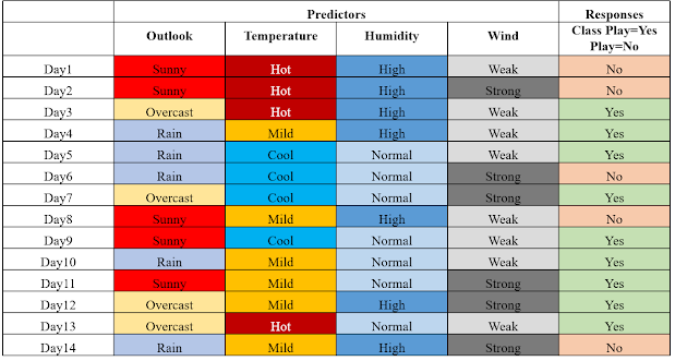
• Let’s build a classifier that predicts whether I should play tennis given the forecast. 
• It takes four attributes to describe the forecast; namely, 

1. the outlook, 
2. the temperature, 
3. the humidity, and 
4. the presence or absence of wind. 

• Furthermore, the values of the four attributes are qualitative (also known as categorical). 
• They take on the values shown below.
• 𝑶𝒖𝒕𝒍𝒐𝒐𝒌 ∈[𝑺𝒖𝒏𝒏𝒚,𝑶𝒗𝒆𝒓𝒄𝒂𝒔𝒕, 𝑹𝒂𝒊𝒏𝒚]
• 𝑻𝒆𝒎𝒑𝒆𝒓𝒂𝒕𝒖𝒓𝒆∈[𝑯𝒐𝒕,𝑴𝒊𝒍𝒅, 𝑪𝒐𝒐𝒍]
• 𝑯𝒖𝒎𝒊𝒅𝒊𝒕𝒚 ∈[𝑯𝒊𝒈𝒉, 𝑵𝒐𝒓𝒎𝒂𝒍]
• 𝑾𝒊𝒏𝒅𝒚 ∈[𝑾𝒆𝒂𝒌, 𝑺𝒕𝒓𝒐𝒏𝒈]
• The class label is the variable, Play and takes the values Yes or No.
• 𝑷𝒍𝒂𝒚∈[𝒀𝒆𝒔, 𝑵𝒐]
• We read-in training data below that has been collected over 14 days

• 
  
  

Classification Phase

Let’s say, we get a new instance of the weather condition, 

 𝑿^′=(𝑶𝒖𝒕𝒍𝒐𝒐𝒌=𝑺𝒖𝒏𝒏𝒚, 𝑻𝒆𝒎𝒑𝒆𝒓𝒂𝒕𝒖𝒓𝒆=𝑪𝒐𝒐𝒍, 𝑯𝒖𝒎𝒊𝒅𝒊𝒕𝒚=𝑯𝒊𝒈𝒉, 𝑾𝒊𝒏𝒅=𝑺𝒕𝒓𝒐𝒏𝒈)  

 that will have to be classified (i.e., are we going to play tennis under the conditions specified by 𝑋^′).

With the MAP rule, we compute the posterior probabilities.

 This is easily done by looking up the tables we built in the learning phase.