Measuring Accuracy Using Cross-Validation

 Measuring Accuracy Using Cross-Validation

        A good way to evaluate a model is to use cross-validation.

        Let’s use the cross_val_score() function to

ü  evaluate our SGDClassifier model,

·       using K-fold cross-validation with three folds.

        Remember that K-fold cross-validation means

ü  splitting the training set into K folds (in this case, three), then

·       making predictions and

·       evaluating them on each fold using

ü  a model trained on the remaining folds.


from sklearn.model_selection import cross_val_score

cross_val_score(sgd_clf, X_train, y_train_5, cv=3, scoring="accuracy")

                        array([0.96355, 0.93795, 0.95615])

ü  Above 93% accuracy (ratio of correct predictions) on all cross-validation folds?

ü  This looks amazing, doesn’t it?

ü  let’s look at a very dumb classifier that just classifies every single image in the “not-5” class:

from sklearn.base import BaseEstimator

class Never5Classifier(BaseEstimator):

def fit(self, X, y=None):

return self

def predict(self, X):

return np.zeros((len(X), 1), dtype=bool)

ü  Can you guess this model’s accuracy?

ü  Let’s find out:

never_5_clf = Never5Classifier()

cross_val_score(never_5_clf, X_train, y_train_5, cv=3, scoring="accuracy")

array([0.91125, 0.90855, 0.90915])

·       It has over 90% accuracy!

·       This is simply because

ü  only about 10% of the images are 5s,

ü  so if you always guess that an image is not a 5,

        you will be right about 90% of the time.

        This demonstrates why accuracy is

        generally not the preferred performance measure for classifiers,

ü  especially when you are dealing with skewed datasets

ü  i.e., when some classes are much more frequent than others.

        Implementing Cross-Validation

ü  Occasionally you will need more control over the cross-validation process than what Scikit-Learn provides off the shelf.

ü  In these cases, you can implement cross-validation yourself. 

Performance Measures

 Performance Measures

        Evaluating a classifier is often significantly trickier than evaluating a regressor.

        There are many performance measures available.

                           i.          Confusion Matrix

                         ii.          True Positive Rate

                       iii.          True Negative Rate

                       iv.          False Positive Rate

                         v.          False Negative Rate

                       vi.          Precision

                      vii.          Recall

                    viii.          Accuracy

                       ix.          F1-Score

                         x.          Specificity

                       xi.          Receiver Operating Characteristic (ROC)

                      xii.          Area Under Curve (AUC)


YouTube Link: https://youtu.be/jL39fMC_I28


Training a Binary Classifier

 Training a Binary Classifier

·       Let’s simplify the problem for now and

ü  only try to identify one digit

—for example, the number 5.

·       This “5-detector” will be an example of a binary classifier,

ü  capable of distinguishing between just two classes,

·       5

·       not-5.


ü  Let’s create the target vectors for this classification task:

y_train_5 = (y_train == 5)

# True for all 5s, False for all other digits

y_test_5 = (y_test == 5)

·       Now let’s pick a classifier and train it.

·       A good place to start is with a

ü  Stochastic Gradient Descent (SGD) classifier,

·       using Scikit-Learn’s SGDClassifier class.

·       This classifier has the advantage of being capable of handling very large datasets efficiently.

·       This is in part because SGD deals with training instances independently, one at a time.

ü  Let’s create an SGDClassifier and train it on the whole training set:

from sklearn.linear_model import SGDClassifier

sgd_clf = SGDClassifier(random_state=42)

sgd_clf.fit(X_train, y_train_5)

ü  The SGDClassifier relies on randomness during training (hence the name “stochastic”).

ü  If you want reproducible results,

        you should set the random_state parameter.

ü  Now we can use it to detect images of the number 5:

sgd_clf.predict([some_digit])

            array([ True])

·       The classifier guesses that this image represents a 5 (True). 


YouTube Link: https://youtu.be/AWI2qUUkPK8


MNIST Dataset Description

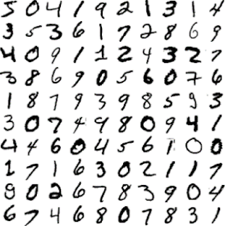
MNIST:

MNIST (Modified National Institute of Standards and Technology):

·       MNIST dataset,

·       which is a set of 70,000 small images of digits handwritten by

ü  high school students

ü  employees of the US Census Bureau.

Each image is labeled with the digit it represents.


Figure 1. Digits from the MNIST dataset


·       This set has been studied so much that it is often called the “hello world” of Machine Learning:

ü  whenever people come up with a new classification algorithm,

ü  they are curious to see how it will perform on MNIST, and

ü   anyone who learns Machine Learning tackles this dataset sooner or later.


ü  Scikit-Learn provides many helper functions to download popular datasets.

ü  MNIST is one of them.

        The following code fetches the MNIST dataset:

from sklearn.datasets import fetch_openml

MNIST = fetch_openml('MNIST_784', version=1)

MNIST.keys()

        dict_keys(['data', 'target', 'feature_names', 'DESCR', 'details', 'categories', 'url']) including the following:

ü  A DESCR key describing the dataset

ü  A data key containing an array with one row per instance and one column per feature

ü  A target key containing an array with the labels


        Let’s look at these arrays:

            X, y = MNIST["data"], MNIST["target"]

X.shape

            (70000, 784)

y.shape

            (70000,)

         There are

ü  70,000 images, and

ü  each image has 784 features.

·       This is because each image is 28 × 28 pixels, and

·       each feature simply represents one pixel’s intensity,

·       from 0 (white) to 255 (black).


·       Let’s take a peek at one digit from the dataset.

·       All you need to do is grab an instance’s feature vector, reshape it to a 28 × 28 array, and display it using Matplotlib’s imshow() function:

import matplotlib as mpl

import matplotlib.pyplot as plt

some_digit = X[0]

some_digit_image = some_digit.reshape(28, 28)

plt.imshow(some_digit_image, cmap="binary")

plt.axis("off")

plt.show()

·       This looks like a 5, and indeed that’s what the label tells us.


y[0]

'5'

·       Note that the label is a string.

·       Most ML algorithms expect numbers, so let’s cast y to integer:

y = y.astype(np.uint8)

·       To give you a feel for the complexity of the classification task,

·       Figure 1 shows a few more images from the MNIST dataset.

·       You should always

ü  create a test set and

ü  set it aside before inspecting the data closely.

·       The MNIST dataset is actually already split into

ü  a training set (the first 60,000 images)

ü  a test set (the last 10,000 images):

X_train, X_test, y_train, y_test = X[:60000], X[60000:],

                                                                                    y[:60000], y[60000:]


·       The training set is already shuffled for us,

ü  which is good because this guarantees that

·       all cross-validation folds will be similar.


·       Moreover, some learning algorithms are

ü  sensitive to the order of the training instances, and

ü  they perform poorly if they get many similar instances in a row.

·       Shuffling the dataset ensures that this won’t happen.


 Youtube Link: 


https://youtu.be/GaVUPdyOSyY


About Machine Learning

Welcome! Your Hub for AI, Machine Learning, and Emerging Technologies In today’s rapidly evolving tech landscape, staying updated with the ...